Porter-Thomas fluctuations

Let’s talk about Porter-Thomas (PT) fluctuations! To do that, we need to start talking about:

The Porter-Thomas distribution

Long story short: The PT distribution is the $\chi^2$ distribution with one degree of freedom ($k = 1$). In nuclear physics we have a central concept, namely the gamma strength function, which is a statistical property of atomic nuclei which describes the nuclei’s gamma decay probabilities. The dipole ($L = 1$) strength function is given by

$$f_{X1}(E_{\gamma}, E_i, j_i, \pi_i) = \dfrac{16 \pi}{9 \hbar^3 c^3}\langle B(X1;\downarrow) \rangle (E_{\gamma}, E_i, j_i, \pi_i) \rho (E_i, j_i, \pi_i).\qquad (0)$$

See p. 230 of Bartholomew et. al. for the general definition. We can re-arrange eq. (0) to get

$$\langle B(Xj_{\gamma}) \rangle (E_{\gamma}, E_i, j_i, \pi_i) = \dfrac{9 \hbar^3 c^3}{16 \pi} \dfrac{f_{Xj_{\gamma}}(E_{\gamma}, E_i, j_i, \pi_i)}{\rho (E_i, j_i, \pi_i)}.\qquad (1)$$

From eq. (1) we see that the GSF $(f)$ is proportional to the mean $B$ value with a proportionality constant of $9 \hbar^3 c^3/(16 \pi \rho)$. The $B$ values deviate from the mean $B$ value by

$$y = \dfrac{B}{\langle B \rangle}$$

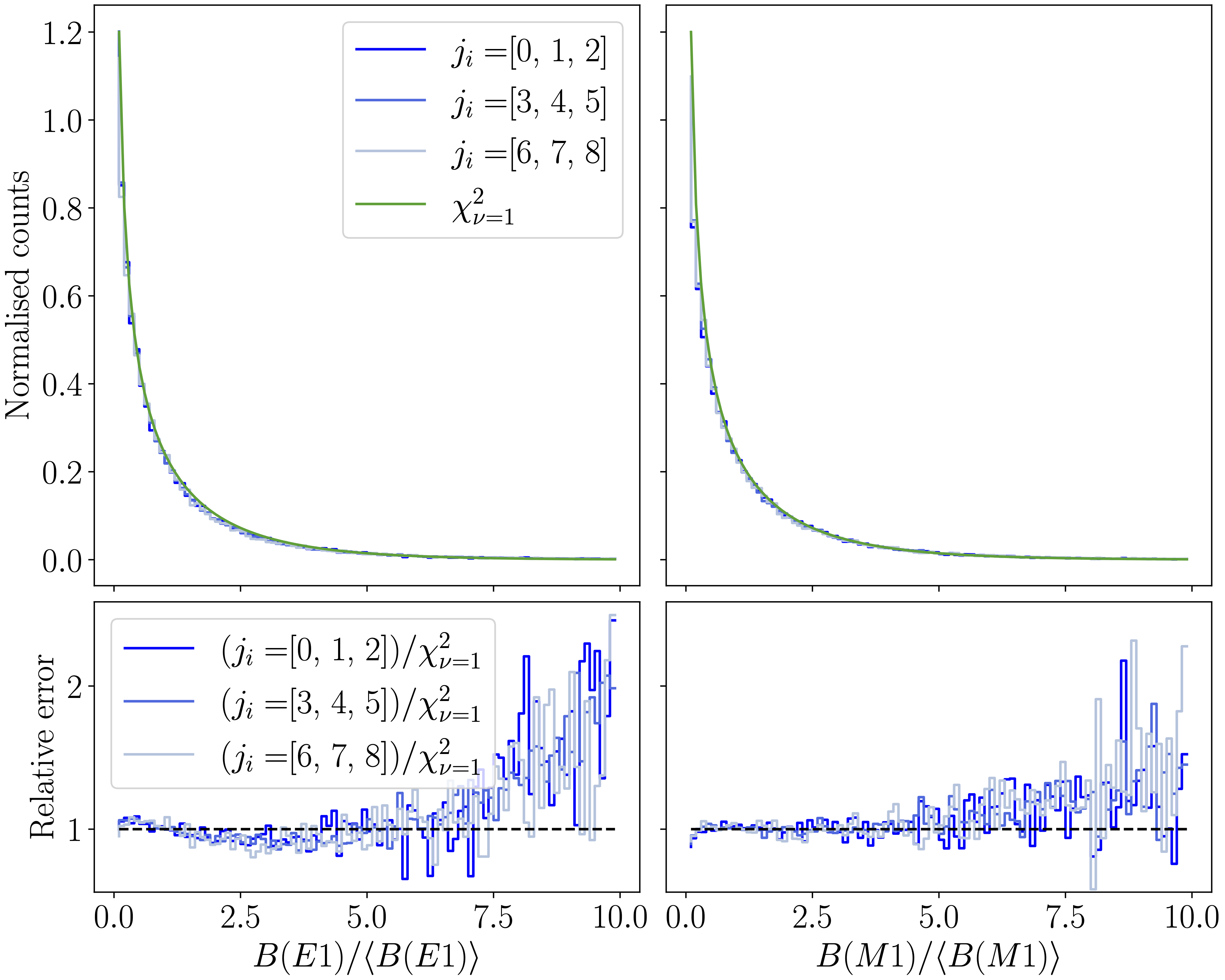
and the distribution of $y$ values are hypothesised to follow the $\chi^2_1$ distribution, aka. the Porter-Thomas distribution. In the following figure we see an example of $B$ values plotted as a histogram and scaled to the height of the PT-distribution to show the resemblance.

Porter-Thomas fluctuations

… is just really a fancy way of saying how much we expect $y$ values to vary. The PDF of the PT distribution is given by

$$g(x) = \dfrac{1}{\sqrt{2 \pi x}}e^{-x/2}, \quad x > 0,$$

with a mean of 1 and a variance of 2. Just check the Wikipedia page if you don’t believe me. Let us now invoke the almighty Central Limit Theorem (CLT)! Let us now draw a value from the PT distribution and we’ll name it $X_1$. Suppose we want to know the sample average

$$\bar{X}_n = \dfrac{X_1 + ... + X_n}{n}.$$

The law of large numbers tells us that the sample average will converge to the expected value $\mu$ as $n$ goes to infinity. The CLT states that as $n$ gets larger, the distribution of $\bar{X}_n$ gets arbitrarily close to the normal distribution with a mean of 1 and a variance of $2/n$ (The PT distribution has a mean of 1 and a variance of 2).

Let us quickly check that this is true! Let’s say that $n = 1000$ and with some quick Python magic:

>>> from scipy.stats import chi2
>>> n = 1000
>>> sum(chi2.rvs(df=1, size=n))/n
1.013582747288161

Pretty close to 1 that is.

>>> draws = [sum(chi2.rvs(df=1, size=n))/n for _ in range(100000)]
>>> np.mean(draws), np.var(draws), 2/n
(0.9999389145605803, 0.002000149052396594, 0.002)

Mic drop?

Now! How can we use this information to determine how much $y$ should vary? And what does vary even mean here? Vary-ance maybe. If $y$ is PT-distributed, then $y$ has a variance of 2. The variance is a measure of dispersion; a measure of how far a set of numbers is spread out from their average value. In mathematical terms, the variance of a random variable $X$ is the expected value of the squared deviation from the mean of $X$:

$$\text{Var}(X) = E[(X - \mu)^2].$$

So maybe what we want is to check that the variance of the $B$ distribution is (close to) 2? We can also draw a bunch of values from the distribution and check that the variance of the mean of all the $n$ draws are indeed equal to $2/n$, as the CLT predicts is true.