Visualising OBTDs

The one-body transition density (OBTD) is used to calculate the transition probability from an initial to a final state:

with the OBTD defined as:

Assume $\alpha$ and $\beta$ ($i$ and $j$ in the list below) to be indices of the orbitals (not the $m$ substates) in the model space, which for sd-pf-sdg are 12 proton orbitals and 12 neutron orbitals. Let’s select a subset of transitions so that we have transitions of gamma energies only within a certain gamma energy interval $[E_\text{min}, E_\text{max}]$. This might for example be the energy interval of the LEE. Let’s also select transitions based on their multipolarities so that we look at only, for example, $M1$ transitions. Transitions of $0^- \rightarrow 1^-$ are within these requirements, and the raw OBTD data for one such transition is listed below. Note that the $M1$ operator has an $L$ and an $S$ term

The file below lists some $L$ matrix element values for vanadium 50 and there is a corresponding file with the $S$ values.

w.f.  J1=  0/2(    3)     J2=  2/2(    1)
 B(L;=>), B(L ;<=)      0.00622     0.00207
 <||L||>      3    1    -0.13590     0.11892

  i  j      OBTD    <i||L||j>  OBTD*<||>
  1  1     0.00244     5.79655     0.01416
  1  2    -0.00012     1.54919    -0.00018
  1  9     0.00000     0.00000     0.00000
  1 10     0.00000     0.00000     0.00000
  1 11     0.00000     0.00000     0.00000
  ...
  

w.f.  J1=  0/2(    3)     J2=  2/2(    1)
 B(L;=>), B(L ;<=)      0.00622     0.00207
 <||L||>      3    1    -0.13590     0.11892

  i  j      OBTD    <i||L||j>  OBTD*<||>
  1  1     0.00244     5.79655     0.01416
  1  2    -0.00012     1.54919    -0.00018
  1  9     0.00000     0.00000     0.00000
  1 10     0.00000     0.00000     0.00000
  1 11     0.00000     0.00000     0.00000
  2  1    -0.00278    -1.54919     0.00430
  2  2    -0.01181     4.64758    -0.05487
  2  3    -0.04737     0.00000     0.00000
  2 10     0.00000     0.00000     0.00000
  2 11     0.00000     0.00000     0.00000
  2 12     0.00000     0.00000     0.00000
  3  2     0.00926     0.00000     0.00000
  3  3     0.00937     0.00000     0.00000
  3 11     0.00000     0.00000     0.00000
  3 12     0.00000     0.00000     0.00000
  4  4    -0.01275     9.62140    -0.12272
  4  5    -0.00304     1.85164    -0.00562
  5  4     0.00360    -1.85164    -0.00666
  5  5     0.00453     8.28079     0.03750
  5  6    -0.00236     0.00000     0.00000
  6  5     0.00402     0.00000     0.00000
  6  6     0.00084     2.58199     0.00217
  6  7    -0.00148     1.15470    -0.00171
  7  6     0.00034    -1.15470    -0.00039
  7  7    -0.00120     1.63299    -0.00196
  8  8    -0.00003    13.98412    -0.00045
  8  9     0.00002     2.10819     0.00005
  9  1     0.00000     0.00000     0.00000
  9  8    -0.00006    -2.10819     0.00013
  9  9     0.00003    12.47219     0.00036
  9 10     0.00000     0.00000     0.00000
 10  1     0.00000     0.00000     0.00000
 10  2     0.00000     0.00000     0.00000
 10  9    -0.00007     0.00000     0.00000
 10 10    -0.00002     5.79655    -0.00010
 10 11     0.00002     1.54919     0.00003
 11  1     0.00000     0.00000     0.00000
 11  2     0.00000     0.00000     0.00000
 11  3     0.00000     0.00000     0.00000
 11 10    -0.00001    -1.54919     0.00001
 11 11     0.00001     4.64758     0.00003
 11 12     0.00001     0.00000     0.00000
 12  2     0.00000     0.00000     0.00000
 12  3     0.00000     0.00000     0.00000
 12 11    -0.00002     0.00000     0.00000
 12 12    -0.00001     0.00000     0.00000
 13 13     0.00045     5.79655     0.00262
 13 14    -0.00046     1.54919    -0.00072
 13 21     0.00000     0.00000     0.00000
 13 22     0.00000     0.00000     0.00000
 13 23     0.00000     0.00000     0.00000
 14 13    -0.00170    -1.54919     0.00264
 14 14     0.00045     4.64758     0.00208
 14 15    -0.00053     0.00000     0.00000
 14 22     0.00000     0.00000     0.00000
 14 23     0.00000     0.00000     0.00000
 14 24     0.00000     0.00000     0.00000
 15 14    -0.00092     0.00000     0.00000
 15 15     0.00015     0.00000     0.00000
 15 23     0.00000     0.00000     0.00000
 15 24     0.00000     0.00000     0.00000
 16 16     0.03272     9.62140     0.31486
 16 17     0.01981     1.85164     0.03669
 17 16     0.00181    -1.85164    -0.00335
 17 17     0.00010     8.28079     0.00084
 17 18    -0.01362     0.00000     0.00000
 18 17     0.02385     0.00000     0.00000
 18 18    -0.07688     2.58199    -0.19852
 18 19    -0.08447     1.15470    -0.09754
 19 18    -0.00732    -1.15470     0.00845
 19 19     0.00582     1.63299     0.00951
 20 20     0.00252    13.98412     0.03530
 20 21     0.00098     2.10819     0.00206
 21 13     0.00000     0.00000     0.00000
 21 20    -0.00036    -2.10819     0.00076
 21 21     0.00018    12.47219     0.00227
 21 22     0.00008     0.00000     0.00000
 22 13     0.00000     0.00000     0.00000
 22 14     0.00000     0.00000     0.00000
 22 21    -0.00000     0.00000     0.00000
 22 22     0.00014     5.79655     0.00084
 22 23    -0.00000     1.54919    -0.00000
 23 13     0.00000     0.00000     0.00000
 23 14     0.00000     0.00000     0.00000
 23 15     0.00000     0.00000     0.00000
 23 22    -0.00008    -1.54919     0.00013
 23 23     0.00000     4.64758     0.00001
 23 24     0.00002     0.00000     0.00000
 24 14     0.00000     0.00000     0.00000
 24 15     0.00000     0.00000     0.00000
 24 23     0.00002     0.00000     0.00000
 24 24    -0.00002     0.00000     0.00000

w.f.  J1=  0/2(    3)     J2=  2/2(    1)
 B(S;=>), B(S ;<=)      0.00022     0.00007
 <||S||>      3    1     0.01050     0.00648

  i  j      OBTD    <i||S||j>  OBTD*<||>
  1  1     0.00244     1.44914     0.00354
  1  2    -0.00012    -1.54919     0.00018
  1  9     0.00000     0.00000     0.00000
  1 10     0.00000     0.00000     0.00000
  1 11     0.00000     0.00000     0.00000
  2  1    -0.00278     1.54919    -0.00430
  2  2    -0.01181    -0.77460     0.00914
  2  3    -0.04737     0.00000     0.00000
  2 10     0.00000     0.00000     0.00000
  2 11     0.00000     0.00000     0.00000
  2 12     0.00000     0.00000     0.00000
  3  2     0.00926     0.00000     0.00000
  3  3     0.00937     1.22474     0.01148
  3 11     0.00000     0.00000     0.00000
  3 12     0.00000     0.00000     0.00000
  4  4    -0.01275     1.60357    -0.02045
  4  5    -0.00304    -1.85164     0.00562
  5  4     0.00360     1.85164     0.00666
  5  5     0.00453    -1.03510    -0.00469
  5  6    -0.00236     0.00000     0.00000
  6  5     0.00402     0.00000     0.00000
  6  6     0.00084     1.29099     0.00109
  6  7    -0.00148    -1.15470     0.00171
  7  6     0.00034     1.15470     0.00039
  7  7    -0.00120    -0.40825     0.00049
  8  8    -0.00003     1.74801    -0.00006
  8  9     0.00002    -2.10819    -0.00005
  9  1     0.00000     0.00000     0.00000
  9  8    -0.00006     2.10819    -0.00013
  9  9     0.00003    -1.24722    -0.00004
  9 10     0.00000     0.00000     0.00000
 10  1     0.00000     0.00000     0.00000
 10  2     0.00000     0.00000     0.00000
 10  9    -0.00007     0.00000     0.00000
 10 10    -0.00002     1.44914    -0.00002
 10 11     0.00002    -1.54919    -0.00003
 11  1     0.00000     0.00000     0.00000
 11  2     0.00000     0.00000     0.00000
 11  3     0.00000     0.00000     0.00000
 11 10    -0.00001     1.54919    -0.00001
 11 11     0.00001    -0.77460    -0.00000
 11 12     0.00001     0.00000     0.00000
 12  2     0.00000     0.00000     0.00000
 12  3     0.00000     0.00000     0.00000
 12 11    -0.00002     0.00000     0.00000
 12 12    -0.00001     1.22474    -0.00002
 13 13     0.00045     1.44914     0.00065
 13 14    -0.00046    -1.54919     0.00072
 13 21     0.00000     0.00000     0.00000
 13 22     0.00000     0.00000     0.00000
 13 23     0.00000     0.00000     0.00000
 14 13    -0.00170     1.54919    -0.00264
 14 14     0.00045    -0.77460    -0.00035
 14 15    -0.00053     0.00000     0.00000
 14 22     0.00000     0.00000     0.00000
 14 23     0.00000     0.00000     0.00000
 14 24     0.00000     0.00000     0.00000
 15 14    -0.00092     0.00000     0.00000
 15 15     0.00015     1.22474     0.00018
 15 23     0.00000     0.00000     0.00000
 15 24     0.00000     0.00000     0.00000
 16 16     0.03272     1.60357     0.05248
 16 17     0.01981    -1.85164    -0.03669
 17 16     0.00181     1.85164     0.00335
 17 17     0.00010    -1.03510    -0.00010
 17 18    -0.01362     0.00000     0.00000
 18 17     0.02385     0.00000     0.00000
 18 18    -0.07688     1.29099    -0.09926
 18 19    -0.08447    -1.15470     0.09754
 19 18    -0.00732     1.15470    -0.00845
 19 19     0.00582    -0.40825    -0.00238
 20 20     0.00252     1.74801     0.00441
 20 21     0.00098    -2.10819    -0.00206
 21 13     0.00000     0.00000     0.00000
 21 20    -0.00036     2.10819    -0.00076
 21 21     0.00018    -1.24722    -0.00023
 21 22     0.00008     0.00000     0.00000
 22 13     0.00000     0.00000     0.00000
 22 14     0.00000     0.00000     0.00000
 22 21    -0.00000     0.00000     0.00000
 22 22     0.00014     1.44914     0.00021
 22 23    -0.00000    -1.54919     0.00000
 23 13     0.00000     0.00000     0.00000
 23 14     0.00000     0.00000     0.00000
 23 15     0.00000     0.00000     0.00000
 23 22    -0.00008     1.54919    -0.00013
 23 23     0.00000    -0.77460    -0.00000
 23 24     0.00002     0.00000     0.00000
 24 14     0.00000     0.00000     0.00000
 24 15     0.00000     0.00000     0.00000
 24 23     0.00002     0.00000     0.00000
 24 24    -0.00002     1.22474    -0.00002

Since there are no transitions between proton and neutron orbitals (gamma decay cannot turn protons into neutrons), we can organise the OBTDs into two 12x12 grids, one grid for protons and one grid for neutrons, for example like this (protons):

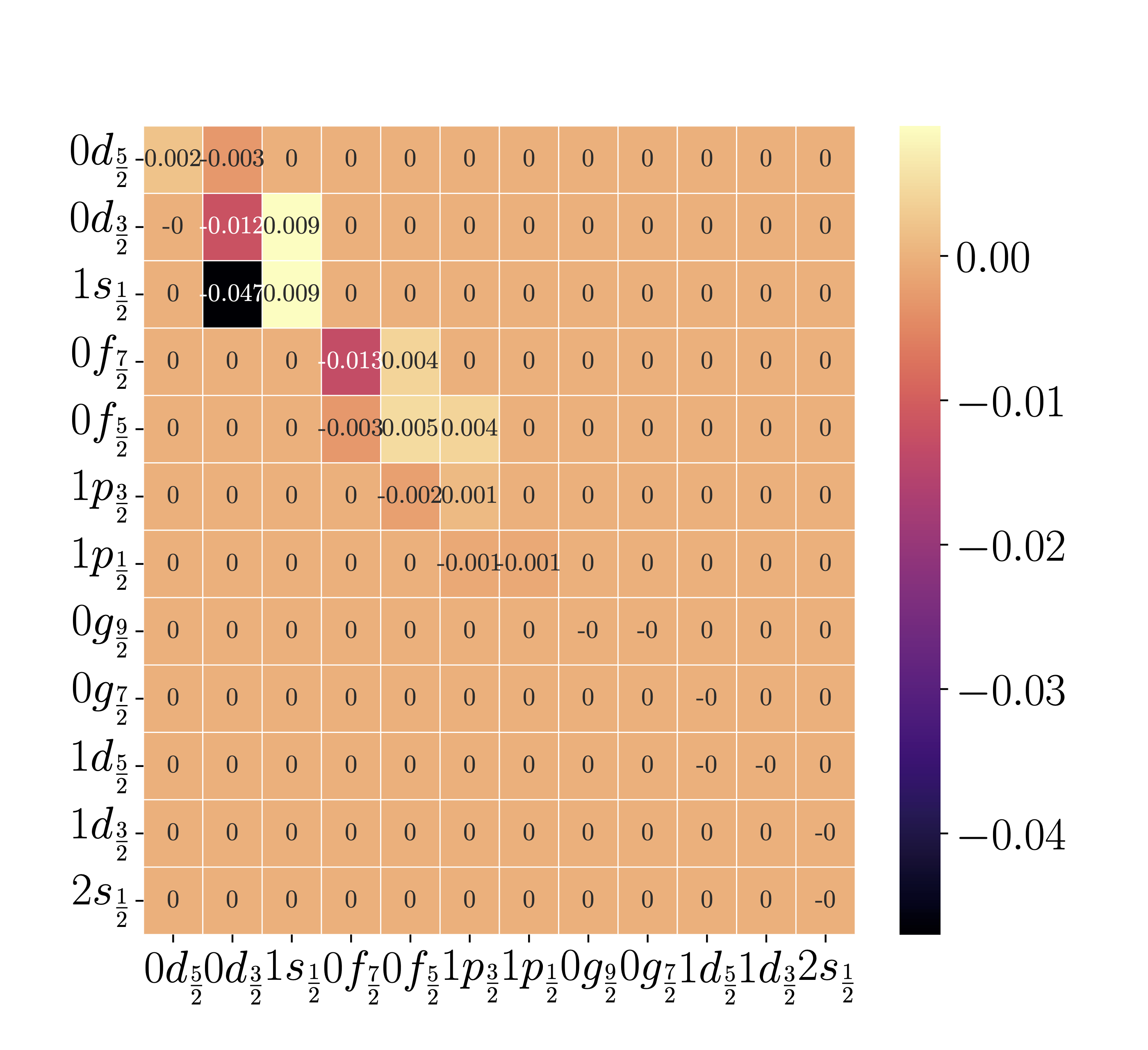
Notice that the OBTD can be negative. If we don’t care about the sign itself, we might take the absolute value of the OBTDs to get a feel of how large the overlap of the initial and final states are given the single-particle transition from $\alpha$ ($i$) to $\beta$ ($j$). One such 12x12 proton OBTD grid can be made for not just this one transition, but one can be made for each of the transitions we selected, which might be tens or hundreds of thousands of transitions. Let’s then consolidate all of the thousands of 12x12 grids into a single 12x12 grid by adding the grids at each grid value. This results in some very large grid values whose magnitude doesn’t really matter; what matters is how large the values are relative to each other. Let’s then normalise by dividing each grid value by the sum of all the grid values and multiply by 100 to express them as a percentage of the sum of all the OBTDs:

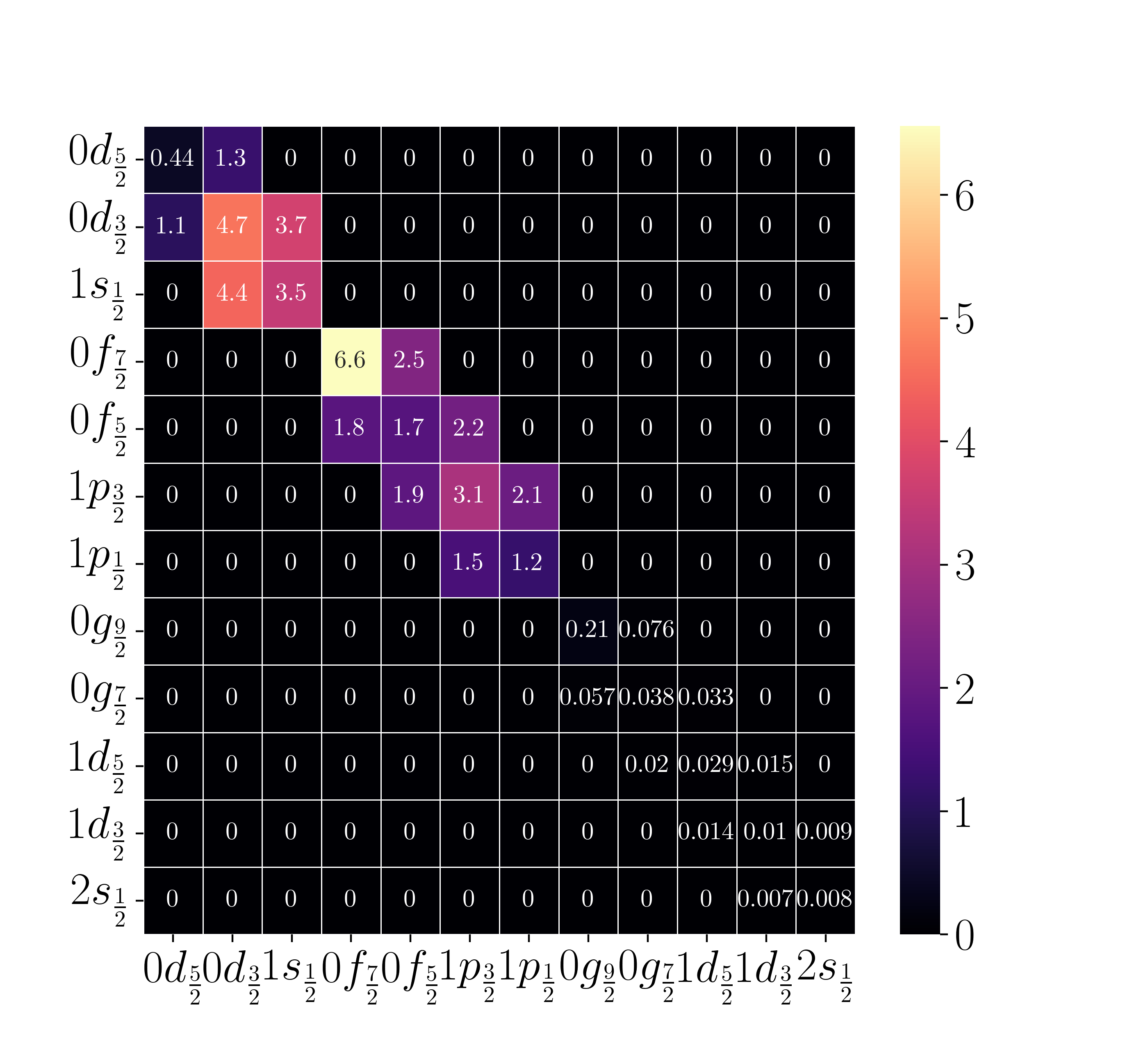
Note that the percentages do not add to 100% because they are normalised to both proton and neutron values and the above plot shows only proton values. The sum of the proton and neutron grid values add up to 100%.

An important consideration to make is that the OBTD eq. (1) has no dependency on any transition operator. The OBTD simply tells us the overlap between the initial and final wavefunctions given a single-particle transition in the initial wavefunction. The OBTD does not care about electromagnetic transition rules, so if we want to consider OBTDs for a subset of transitions with an $M1$ characteristic we need to do some filtering.

Note that the $M1$ operator in eq. (2) consists of an $L$ and an $S$ term, the values for $L$ and $S$ for a single transition are given in the above lists. We see that in some cases a non-zero OBTD value has corresponding $L$ and $S$ values which are zero. In such a case, I think it would be wrong to include that OBTD value in the 12x12 grid since its contribution is zeroed by transition rules. Here I’m assuming that the angular momentum and parity transition rules manifest as the $L$ and $S$ terms being zero. If you look at eq. (0), where else could the transition rules come into play? There are only two terms.

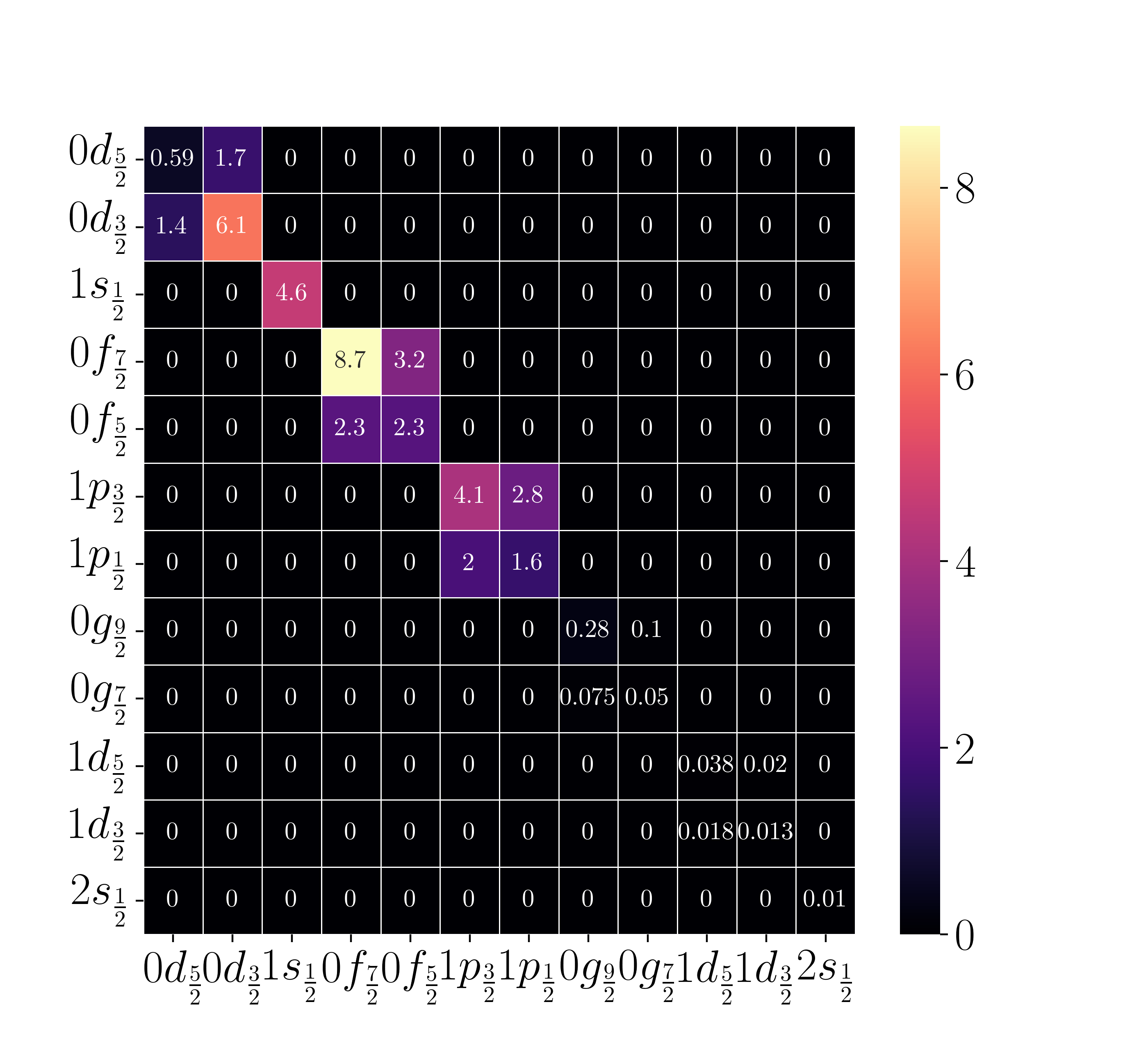
Now what can we say about these two latest 12x12 grids… First, the single-particle transitions seem to respect the transition rules for $M1$ transitions. Recall that $M1$ transitions have no change in parity from the initial to the final state which means that the only allowed single-particle transitions are within each major shell. We can clearly see block structures within $sd$, $pf$, and $sdg$. Second, $M1$ transitions allow only $\Delta j = 1$, recall the rule

which means that, for example, a single-particle transition from $s1/2$ to $d5/2$ has a minimum $\Delta j$ of 2, and consequently that this single-particle transition is illegal for $M1$ transitions.

We can see that even before explicitly respecting the $M1$ transition rules by skipping OBTDs where $L$ and $S$ are zero, the OBTDs in the 12x12 grid already agree with $\Delta j = 1$ and $\Delta \pi = \text{no}$. This probably comes from the fact that I already made a selection of transitions which are $M1$ transitions, but just because I selected $M1$ transitions does not mean that all single-particle transitions within the $M1$ transitions (eq. (0)) are allowed.

A still open question to me is why the $1s1/2 \rightarrow 0d3/2$ OBTDs disappeared when

allows $M1$ transitions…

Parity

Vanadium 50 has 23 protons and 27 neutrons and is a so-called odd-odd nucleus. Since there is an even number of nucleons, and since the fermi surface for protons and neutrons both are in the same major shell ($pf$), and since parity is a multiplicative quantum number, then the ground state parity of 50V is positive. The ground state parity is also called the natural parity of 50V.

Below are two 12x12 grids, both for protons, which are filtered by the parity of the initial level in the transitions (since these are $M1$ the final parity will be the same as the initial). To the left we have positive parity (aka. natural parity for 50V) and to the right we have negative parity.

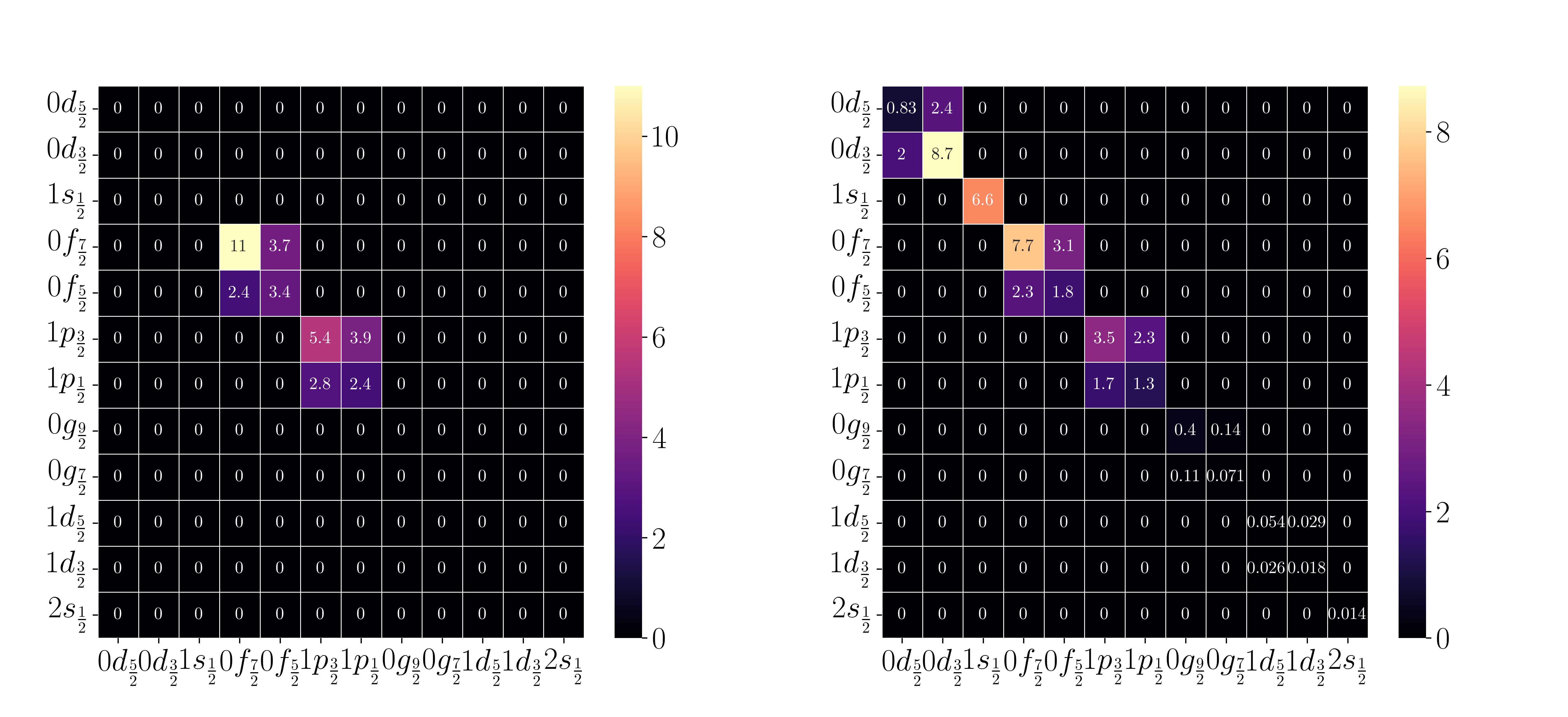
Let’s start with the natural parity (left): The only non-zero OBTDs are within the $pf$ shell which agree with my expectations. First, the fermi surface for both protons and neutrons is in the $0f7/2$ orbital so we expect a lot of action inside the $pf$ shell. Second, since the $sd$ shell is completely full, and since protons and neutrons are fermions which means that permutations don’t matter, the $sd$ shell is completely locked as long as there are no $\hbar \omega$ excitations (excitations across a major shell gap). If we allow an $\hbar \omega$ excitation from $sd$ to $pf$ then we change the parity to negative and hence it will not show up in the left 12x12 grid. If we excite two nucleons from $sd$ to $pf$ we will get back to the natural parity, but the calculations we are looking at are restricted to a $1 \hbar \omega$ truncation, meaning that only one nucleon can be excited across a major shell gap at any time. Consequently we should see OBTDs only in the $pf$ shell for the natural parity states.

Now let’s take a look at the un-natural parity (right): Here we see action in all the major shells which makes sense. For these OBTDs we consider only states where one nucleon has been excited either from $sd$ to $pf$, or from $pf$ to $sdg$. $\hbar \omega$ excitations are needed to change the parity, and while any odd number of $\hbar \omega$ excitations would suffice, the truncation of the calculations allow only one. Exciting one nucleon from $sd$ to $pf$ opens up for movement in the $sd$ shell and we can clearly see that stuff is going on down there. Similarly, exciting one nucleon from $pf$ to $sdg$ opens up for a lot of movement in the $sdg$ shell, but since those orbitals are quite far above the fermi surface, and thus energetically unfavourable, the OBTDs are relatively low.

Now, what I cannot yet wrap my head around is the fact that all the non-zero OBTDs are strictly within orbit partner orbitals (aka. orbitals with the same orbital angular momentum $l$). For example, $0d3/2 \rightarrow 1s1/2$ is legal both with regards to parity and with regards to angular momentum, but after removing OBTDs where the $L$ and $S$ terms are both zero, OBTDs for that transition (and other seemingly legal ones too) have completely disappeared…

As a function of B

Another possible interesting aspect of the OBTDs is to see the orbitals’ contributions for different transition strengths, $B$ values in this case. You might say that strong transitions are the most important ones, but on the other hand the weaker transitions are by far more numerous, as is evident from the following plot of B/mean(B) distributions:

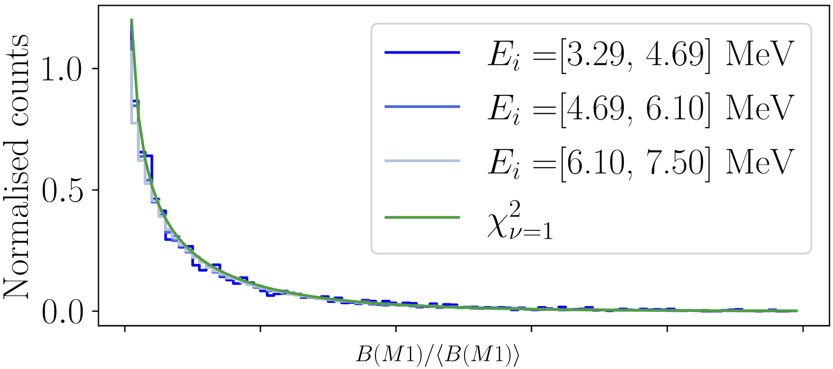
A central part of gamma decay theory and the GSF in particular is that the $B$ values follow the $\chi^2$ distribution with one degree of freedom. In this field the $\chi^2$ distribution is usually called the Porter-Thomas distribution. In the above figure, there are three $B$ distributions using transitions drawn from different $E_i$ (initial state’s excitation energy) ranges, the reason for which is to show that the Porter-Thomas distribution emerges regardless of the detailed structure of the initial states. Closely related to the Brink-Axel hypothesis.

Anyway, looking at how the OBTD for a specific single-particle transition develops as a function of transition strength might provide some insight. In the following figure we see exactly that for all the non-zero single-particle transitions in the $sd$ and $pf$shell for protons (left) and neutrons (right). In the above 12x12 grid for negative parity we see that there are non-zero OBTDs in the $sd$ and $sdg$ shells too so don’t expect the numbers in the current figure to completely add up to 100%:

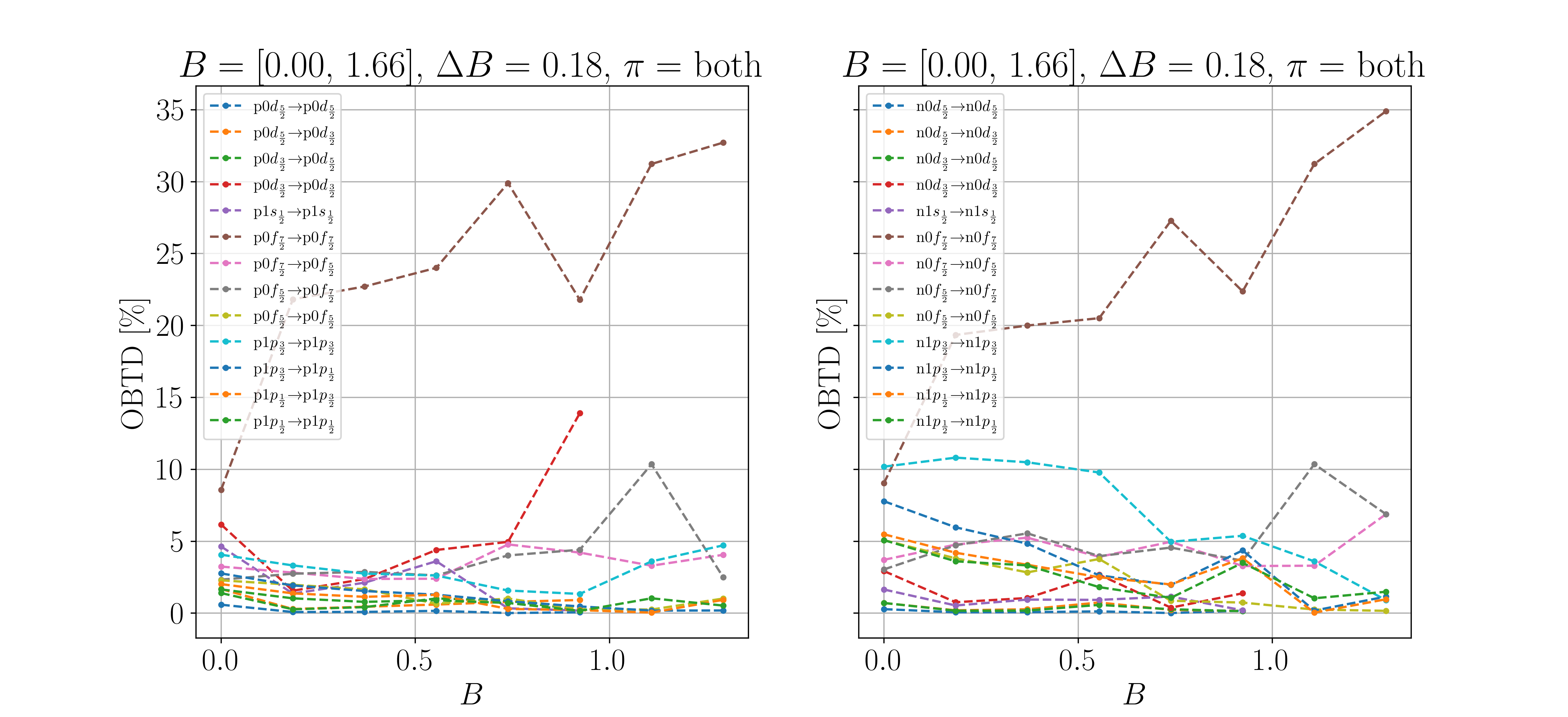
Well, it is apparent that $0f7/2 \rightarrow 0f7/2$ is the main contributor for both protons and neutrons. Seems also to follow the same trend for protons as for neutrons. At the mid-high $B$ values $p0d3/2 \rightarrow p0d3/2$ makes a valiant attempt at reaching $p0f7/2 \rightarrow p0f7/2$ but at higher $B$ values there is no more OBTD data for it. Judging by the continued increase of $0f7/2 \rightarrow 0f7/2$ I’d say that $p0d3/2 \rightarrow p0d3/2$ does not take over as the most dominant at the largest $B$ values.

For good measure, here are the same figures but parity separated:

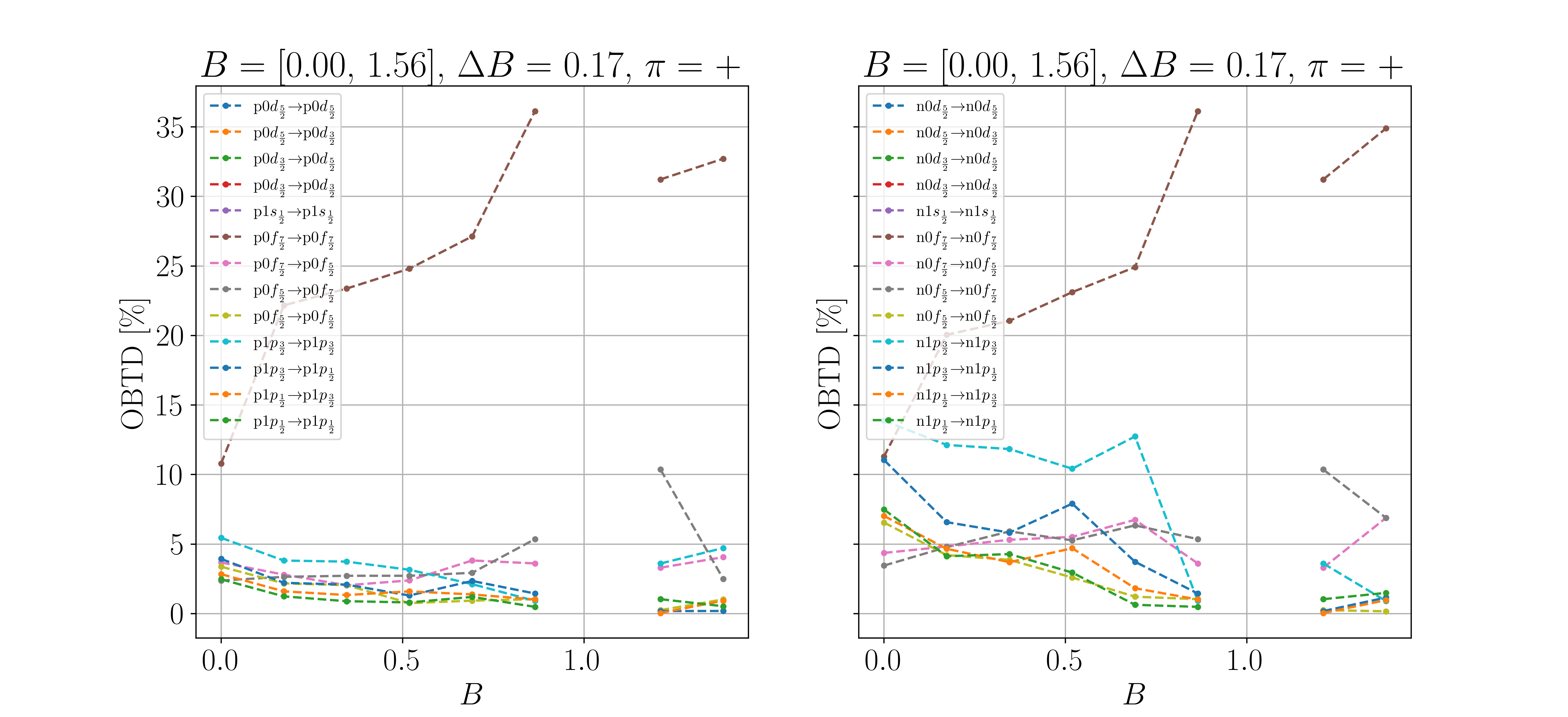
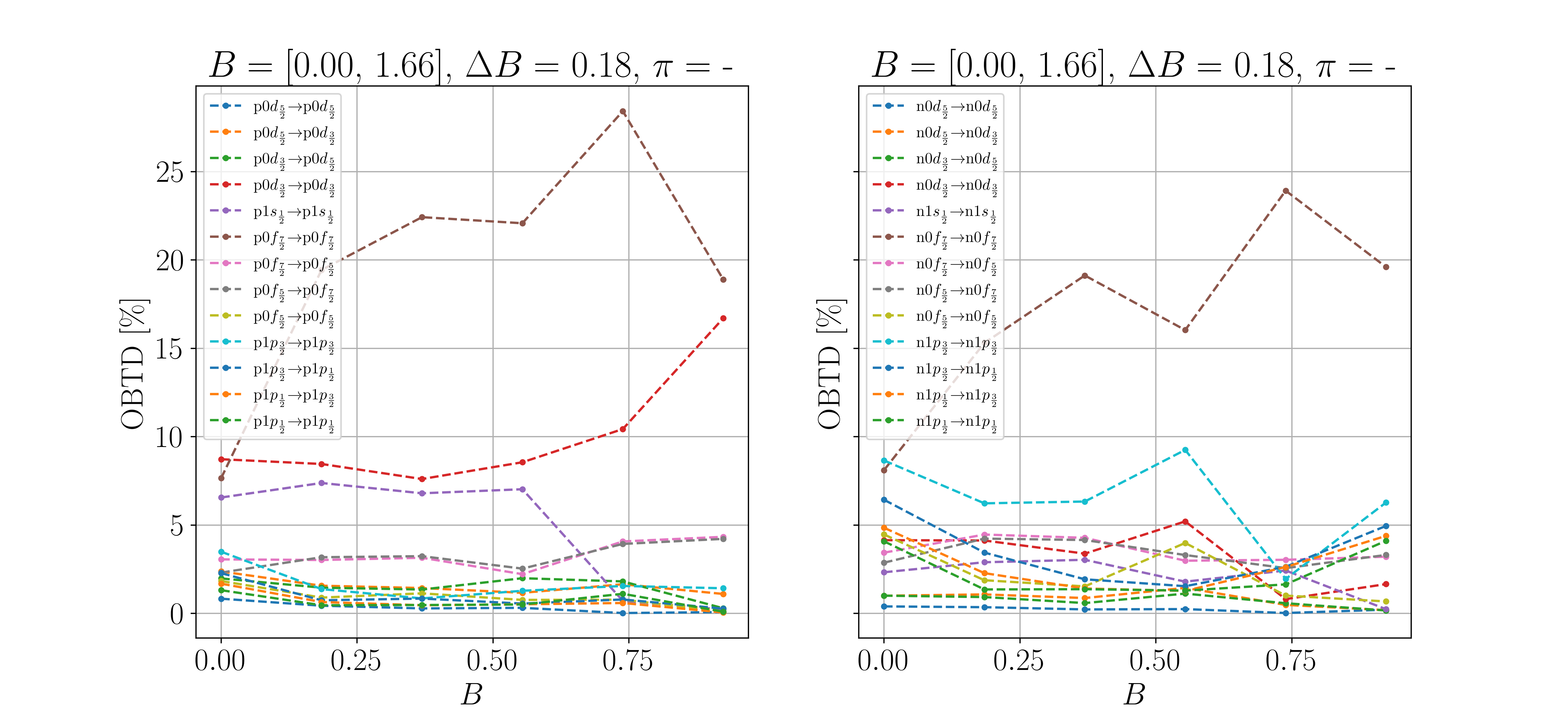
Maybe the most striking feature is that the natural parity has a gap around $B = 1$. There simply are no transitions of that strength under the selection I have done. For the negative parity however, there are transitions for all $B$ values in the range.

$0f7/2 \rightarrow 0f7/2$ asserts dominance in all the cases, however a bit less for negative parity. For protons and positive parity, $0f7/2 \rightarrow 0f7/2$ is completely dominating. For neutrons and positive parity we actually see that $1p3/2 \rightarrow 1p3/2$ starts as the most dominant at the lowest $B$ values, holds at 10% - 13% before falling towards zero at the highest $B$.

As for protons and negative parity, we see that $0d3/2 \rightarrow 0d3/2$ starts with a slight lead, is steady at just under 10%, and seems to increase at the highest $B$ value approaching $0f7/2 \rightarrow 0f7/2$. I do wonder what would happen at even larger $B$ values… With neutrons and negative parity we see that $0f7/2 \rightarrow 0f7/2$ dominates less and that $1p3/2 \rightarrow 1p3/2$ also makes an appearance, as with the natural parity case.

Now my next endeavor will be to modify the OBTD files as to artificially remove the contributions from certain orbitals and then plot the GSF to see if the LEE is affected. Stay tuned!